Advanced Tutorial
|
This advanced tutorial introduces the concepts of asymmetrically loaded plaques, Central AXis (CAX) vs Tumor AXis (TAX) tables, Meridian and Equatorial 2D dosimetry planes, 3D dose calculations and 3D appearance.
|
|
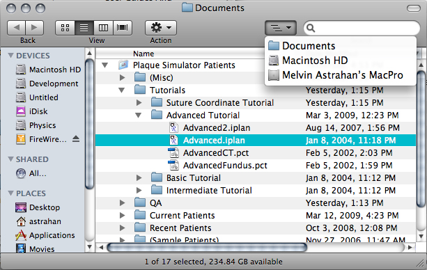
1. The advanced tutorial file Advanced.iplan can be found in the Tutorials folder which is located in the Plaque Simulator Patients folder which is in the Documents folder at the root level of your system hard drive. These files and folders were installed as part of your original installation or update of Plaque Simulator. Copies are also on your distribution CD and the latest versions are available via internet download from the Plaque Simulator website www.eyeplaque.com.
|
|
|
This example uses the same images as the intermediate tutorial. The difference is that an asymmetrically loaded notched 18 mm COMS style plaque has been used instead of the standard 12 mm COMS plaque. If this were a actual patient, there would be no clinical advantage to doing this, the purpose here is purely to illustrate some features of the software.
|

|
|
The plaque has been asymmetrically loaded in the slots which cover the tumor base.
|

|
|
Resulting in this dose distribution on the retinal surface.
|

|
|
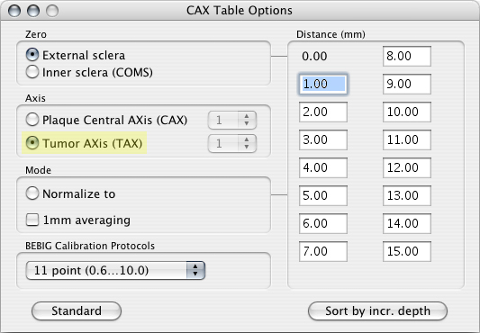
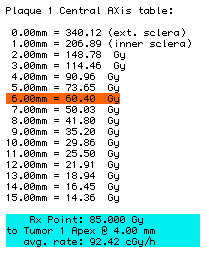
In the basic and intermediate tutorials the Prescription window was set to display the Central AXis (CAX) table. In this example, the plaque CAX does not well represent dose in the tumor.
|
|
|
|
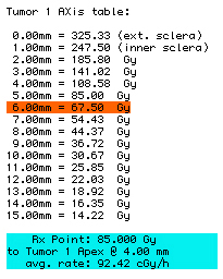
Illustrated here are the points of the two "axis" tables. The correct table to use in this situation would be the Tumor AXis (TAX) table.
|
Central AXis (CAX) points.
|
Tumor AXis (TAX) points.
|
|
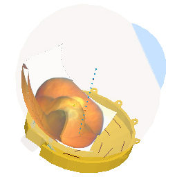
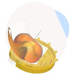
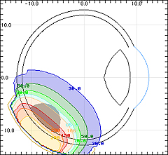
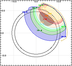
Illustrated here are meridian and equatorial 2D isodose plots and 3D views of the planes corresponding to these plots. 2D isodose surfaces are selected and positioned from the Dosimetry window.
|
Surface 1, Meridian Plane.
|
Surface 2, Equatorial Plane (offset from equator)
|
|
|
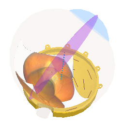
Meridian Plane.
|
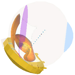
Equatorial Plane (offset from equator)
|
|
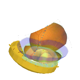
These examples of Setup window views illustrate rendering of 3D isodose surfaces. Calculating the 3D dose matrix is a simple two step process: From the Dosimetry menu, first Allocate the 3D Matrix and then Calculate the 3D Matrix.
The 3D isodose surface is selected from the radio buttons in the 3D column of the Isodose window.
To render the 3D isodose surface use this button  in the Setup window. in the Setup window.
|
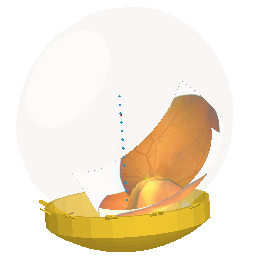
3D isodose off.
|
3D isodose on, translucent.
|
|
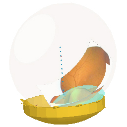
These examples of Setup window views illustrate rendering of 3D isodose surfaces and the retinal dose surface.
To render the retinal dose surface use this button  in the Setup window. in the Setup window.
|
translucent + retinal surface.
|
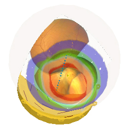
translucent + retinal surface.
|
|
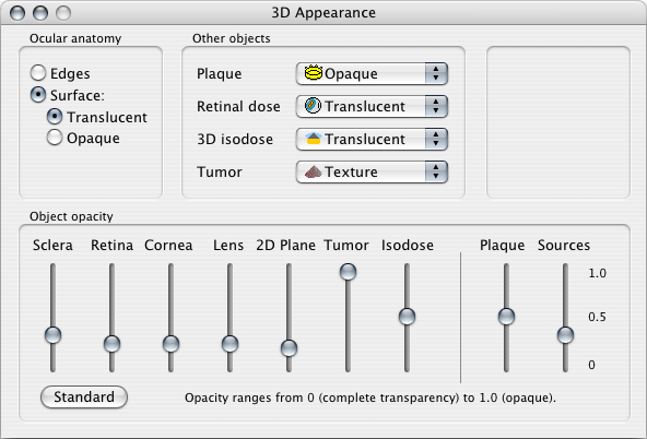
The appearance of 3D objects in the Setup window is controlled from the 3D Appearance window. This window is opened by clicking on the appearance button located along the bottom of the Setup window.

|
|
Guide Contents