A Quality Assurance (QA) procedure has been implemented to assure that the software is operating correctly. You should run this QA test at installation and after you install a software upgrade.

From the Setup window select Open Patient... from the File menu and use the MacOSX file navigation services to find and open the Quality Assurance V6.iplan6.

Step 1: by:

Date performed: ___ / ___ / ______

In the PS models of COMS plaques, linear sources are assumed to be oriented tangent to a concentric sphere of the silicone seed carrier with their centers 1.4 mm from the face (concave surface) of the carrier.

The V6 QA file includes a COMS 14 mm plaque with a single model TG43U1 6711 I-125 source of strength 1.0 mCi (calibrated to the plaque insertion date and time) in the central slot of the seed carrier which is centered on the plaque's Central AXis at coordinates (-1.40,0.00,0.00).

The Plaque window should look like this:

Step 2a: by:

Date performed: ___ / ___ / ______

The plaque is centered under a conical tumor that has a 10 mm diameter circularly shaped base. Plaque Simulator follows the COMS convention of measuring tumor height from the inner sclera which is assumed to be 1 mm thick, so the apex of this 7.6 mm tall tumor will be 10 mm perpendicular to the axis of the central source in the carrier. The PS prescription (Rx) point is set at the apex of the tumor.

Resize the Planar Dosimetry window to 400x400 pixels by clicking the window size control at the lower left corner and selecting 400x400 from the sheet. Click the OK button to close the sheet.

The Planar Dosimetry window should look like this:

Step 2b: by:

Date performed: ___ / ___ / ______

Widen the Prescription window slightly by dragging the lower right corner so you can see all of the toolbar controls.

The dose calculation algorithm controls in the toolbar from left to right should be set to:

• Source geometry = Point (vs linear)
• Isotropy = Isotropic (vs anisotropic)
• Carrier disabled
• Gold scatter disabled
• Collimation type = Lipped (vs Slotted)
• Shell collimation disabled
• Air scatter disabled
• Calculation algorithm set to PS (vs COMS)

The Duration (dose integration time) is one hour. The source activity has been calibrated to 1.0 mCi on the date and time of implant insertion. This simple setup can be checked against a TG-43 hand calculation.

An initial dose rate of 1.234 cGy/h should be displayed for both the Rx point, the Tumor 1 apex at 7.6 mm from the inner sclera, which is at 8.6 mm from the face of the plaque seed carrier (in the Central AXis table) and therefore 1 cm from the linear axis of the seed which is offset 1.4 mm deep into the seed carrier.

This value represents the basic TG43 formalism

where the seed active length L = 3 mm, and for this calculation geometry r = 1 cm, r₀ = 1 cm, θ = 90° and θ₀ = 90°, so...

• air kerma strength S_K = 1.0 mCi multiplied by the apparent activity to air kerma strength conversion factor (1.27)
• the TG43 defined dose rate constant Λ for the model 6711 seed in water = 0.965
• geometry function G_L(r₀,θ₀) = 0.9926 (this factor removes the linear geometry effect from Λ)
• geometry function G_L(r,θ) for a point source is 1/r² = 1.0
• the radial dose function g(r) = 1.0 at r = 1 cm (by definition)
• and the 2D anisotropy function F(r,θ) = 1 because the source is considered to be isotropic in this calculation

The complete equation is (1.0 x 1.27) x 0.965 x (1.0 / 0.9926) x 1 x 1 = 1.234.

Step 3: by:

Date performed: ___ / ___ / ______

In this step you will first test that the implant duration and units functions are working correctly

You will then test that the QA_Check function, which is coded independently of the main PS dosimetry engine, is returning the same result as the PS dosimetry engine when the PS engine is configured for an isotropic point source in water.

Note: the QA_Check function and the PS dosimetry engine do, however, share the same radionuclide physics data.

You will then return the Prescription window to its previous settings.

• In the Plaque #1 removal controls group, change the duration to 168 hours by typing or clicking the 1 Week button.
• In the footer controls along the botom of the window, click the Rx units button and change the display to Gy in the popup menu.
• Confirm that the prescription bar and central axis table units change to Gy.

• In the Documents window, select the QA document.
• The QA_Point dose (which is calculated using the PS dosimetry engine) and QA_Check dose (which is calculated using an independent function) should be exactly the same.
• Confirm that the ratio Point/Check = 1.
• In the Prescription window, return to a duration of 1 hour and units of cGy/hr.
• Confirm that the prescription bar and central axis table units return to cGy/hr. The Prescription window should once again look as it did in step 3 above.

Step 4: by:

Date performed: ___ / ___ / ______

From the dosimetry menu select Calculate 2D Matrices.

The Isodose window should be configured as illustrated below with isodose normalization enabled and set to 1.0 at the prescription (Rx) point.

Step 5: by:

Date performed: ___ / ___ / ______

For a more comprehensive QA check, click the Point control in the Prescription window toolbar. This enables linear sources and the control changes to read "Linear". Treating the source as linear will reduce the dose rate by approximately 1% at 10 mm on the central axis compared to the point geometry calculation.

Next, enable anisotropy correction by clicking the Isotropy control in the Prescription window toolbar. Dose rate on the central axis should be unaffected because F(r,θ) equals 1.0 at 0 degrees (ie perpendicular to the seed axis at its center). The dose rate at off-axis anatomic points of interest such as macula and optic disc will change.

Next, enable Carrier correction by clicking the Carrier control menu arrows in the Prescription window toolbar and select T(r,d,μ). Correcting for attenuation in the silicone carrier will reduce the dose rate by approximately 13% at 10 mm on the central axis. The dose rate at off-axis anatomic points of interest such as macula and optic disc will also change.

Activating Shell collimation should have no effect on the central axis table since central axis points are never collimated by the shell of a COMS plaque. The dose rate at off-axis anatomic points of interest may change depending upon the plaque location on the eye. Toggling between Slotted and Lip collimation should have no effect since a COMS plaque does not have collimating slots.

Widen the Prescription window slightly by dragging the lower right corner so you can see all of the toolbar controls.

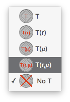
Change the dose calculation algorithm controls in the toolbar from left to right to:

• Source geometry = Linear (vs point)
• Isotropy = Anisotropic (vs isotropic)
• Carrier enabled in mode T(r,d,μ)
• Gold scatter disabled
• Collimation type = Lipped (vs Slotted)
• Shell collimation enabled
• Air scatter disabled
• Calculation algorithm set to PS (vs COMS)

An initial dose rate of 1.071 cGy/h should be displayed for both the Rx point, the Tumor 1 apex at 7.6 mm from the inner sclera, and at 8.6 mm (from the face of the plaque) in the Central AXis table.

This value represents the basic TG43 formalism

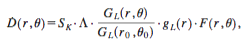
where the seed active length L = 3 mm, and for this calculation geometry r = 1 cm, r₀ = 1 cm, θ = 90° and θ₀ = 90°, so...

• air kerma strength S_K = 1.0 mCi multiplied by the apparent activity to air kerma strength conversion factor (1.27)
• the TG43 defined dose rate constant Λ for the model 6711 seed in water = 0.965
• geometry function G_L(r₀,θ₀) = 0.9926 (this factor removes the linear geometry effect from Λ)
• geometry function G_L(r,θ) for a linear source (instead of a point source as in the earlier example)
• the radial dose function g(r) for r = 1 cm
• and the 2D anisotropy function F(r,θ) at r=1cm, θ=90° for this seed model.

plus additional PS extensions (to the TG43 equation) whch account for

• carrier attenuation which accounts for the greater attenuation (compared to homogeneous water) in about 1 mm of silastic material which radiation leaving the seed must pass through en route to the dose calculation point
• shell collimation which for this particular dose calculation point should have no effect because there are no collimating surfaces between the tumor apex and the seed.

Step 6: by:

Date performed: ___ / ___ / ______

From the dosimetry menu select Calculate 2D Matrices.

The Isodose window should be configured as illustrated below with isodose normalization enabled and set to 1.0 at the prescription (Rx) point.

Step 7: by:

Date performed: ___ / ___ / ______

From the Setup Window click the Offset button

to open the Plaque Offset window.

• Set the offset to 2 mm
• Set Y rotation to 15 deg.
• From the dosimetry menu select Calculate 2D Matrices.

After offsetting and wobbling the plaque, and recalculating the 2D dose matrices, the dose and dose rate at the Rx point (tumor apex) may change significantly. The calculation of collimation should rotate with the plaque, while isodose lines plotted in the Planar Dosimetry window should remain normalized to the tumor apex.

Note: all PS dosimetry calculations are performed in absolute eye coordinates because multiple plaques are allowed, and some complex formuli are closely approximated using lookup tables in order to accelerate the dose calculation. When a plaque is rotated (wobbled) away from its default orientation tangent to the sclera at its center, a few of the central axis table values close to the plaque's face, where the dose gradient is very steep, might change insignificantly due to rounding differences into the lookup tables.

This completes the V6 quality assurance procedure.

If any of your results while following this QA procedure do not match the illustrated expected results, please discontinue use of the software, make screen captures of your results and send the screen captures as attachments with an explanatory email to the licensed distributor and software developer. Contact information may be found in the contact section of the About window.

Step 8: by:

Date performed: ___ / ___ / ______