Manual Calibration

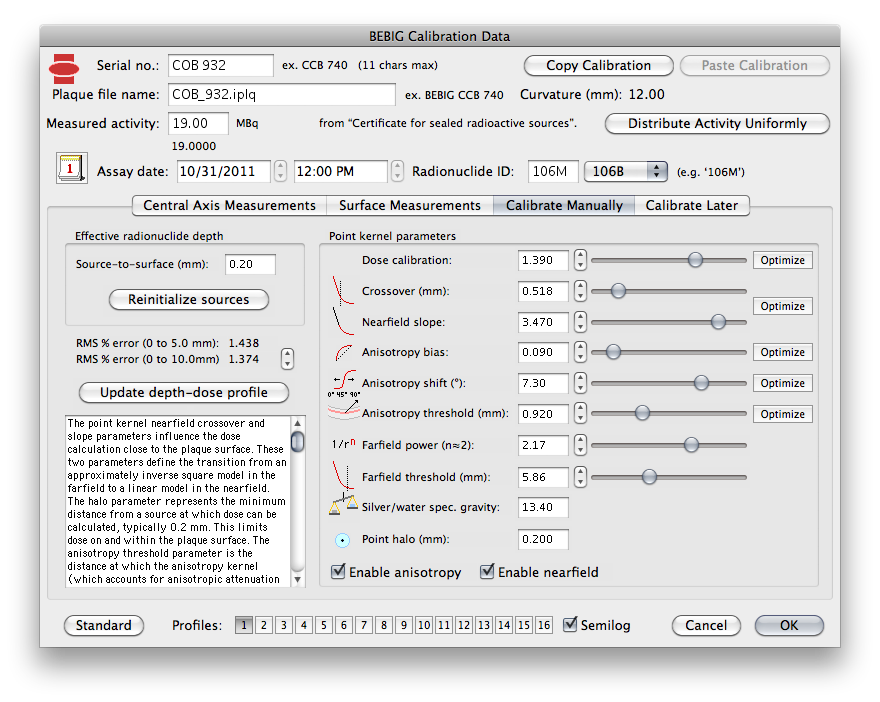
Manually Fine-Tuning the Calibraton

After the automated optimization and surface annealing processes are complete you will need to manually fine tune the model parameters.

Click the Calibrate Manually tab. Adjust the parameters using the sliders followed by the bumper arrows to minimize the RMS% error of the fit of the central axis profile to the measured data over the range 0..10mm.

Manual fine-tuning is an iterative process. Begin by adjusting the Dose Calibration slider until the dose profile curve passes through the 5 mm measurement point.

Next, adjust the Crossover slider to minimize the RMS error in the range 0..5 mm.
Next, adjust the Nearfield slope slider to minimize the RMS error in the range 0..5 mm.
Next, adjust the Anisotropy shift slider to minimize the RMS error in the range 0..5 mm.
Next, adjust the Anisotropy threshold slider to minimize the RMS error in the range 0..5 mm.
Next, adjust the Farfield threshold slider to minimize the RMS error in the range 0..10 mm.
Next, adjust the Farfield power slider to minimize the RMS error in the range 0..10 mm.
Next, adjust the Dose Calibration slider to minimize the RMS error in the range 0..5 mm.

Repeat steps 2-8 until the RMS error over the range 0..10 mm can no longer be reduced. Optional: try varying the order of the steps to see if any further reduction is possible.
Lastly, adjust the Anisotropy bias slider to further minimize the RMS error in the range 0..5 mm.
Repeat steps 2-10 until the RMS error in the range 0..10 mm can no longer be reduced.
It is typically possible to achieve a central axis RMS error of under 2% over the range 0..10mm.
You may optionally return to the Surface Measurements section and repeat the simulated annealing followed by repeated manual fine-tuning to see if the RMS error between calculated and surface measurements can be further reduced.

Below are the results of 2 passes of simulated annealing followed by manual fine-tuning for this COB example plaque.

For this example, after the first pass of simulated annealing of the surface strength distribution, followed by a fine tuning, a central axis RMS % error of 1.55 was achieved over the range 0..10 mm.

After a second pass of simulated annealing followed by a second pass of fine tuning, a central axis RMS % error of 1.37 was achieved over the range 0..10 mm.

Click the OK button to proceed to save the plaque file.

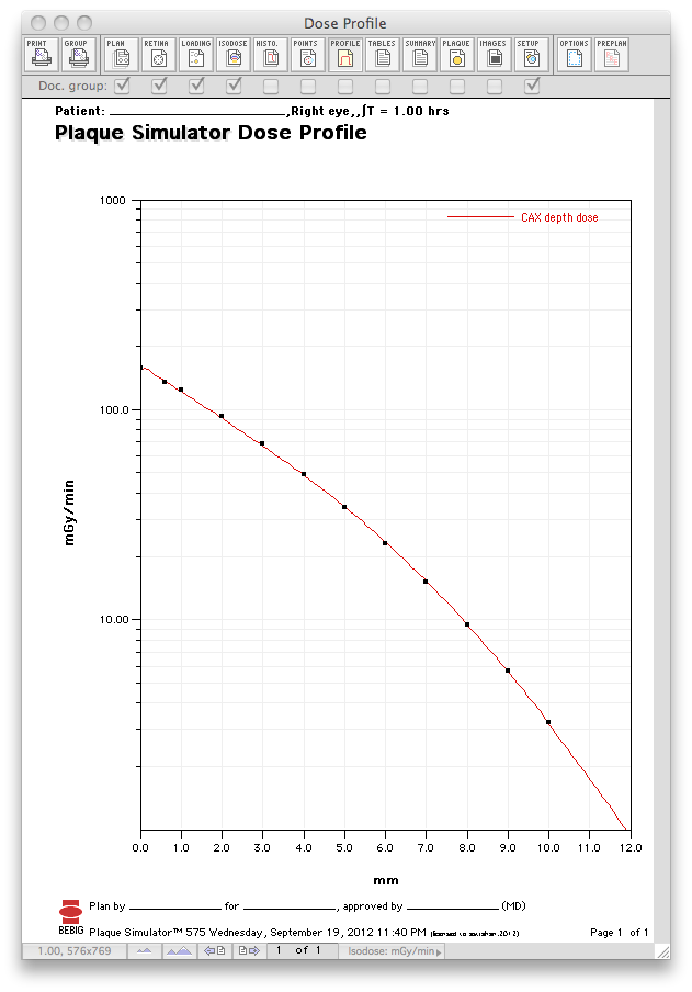
Below are sample isodose calculations for this plaque with its notch up against the optic nerve. All dosimetry has been normalized to 1.0 on the central axis of the plaque at 1 mm from the surface of the plaque, the same normalization point as the BEBIG near-surface measurements. Please note that the BEBIG points are normalized to a value of 100 whereas the PS isodose lines are normalized to 1.0.

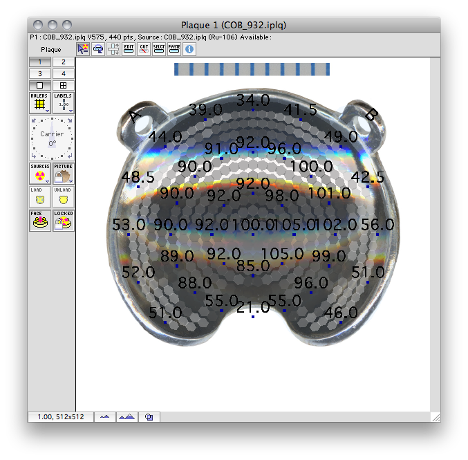
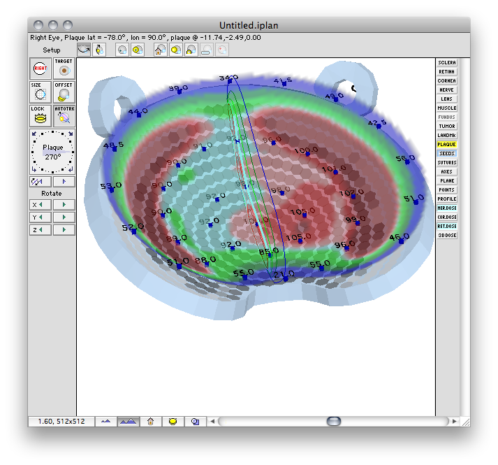
The BEBIG surface measurements and nonuniform distribution of patch-source (gray hexagons) strength as seen in the Plaque Loading window.	3D view of the normalized isodose distribution on the retinal surface, isodose lines on the meridian plane, and the normalized surface measurements.
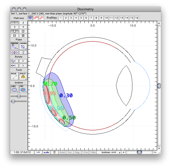
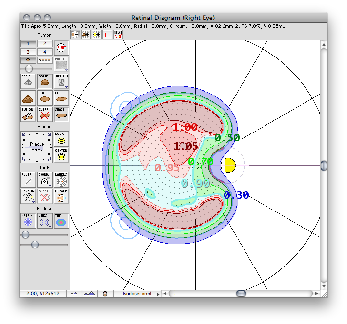
Normalized isodose distribution on the 9 o'clock meridian plane which passes through the nerve, the notch and the plaque center.	Normalized isodose distribution on the retinal diagram.