In PS version 6.8.6 and later you will want to create a folder named DCMTK which contains an HFS AXIAL orbital study series of 16-bit MONOCHROME DICOM files with little endian Transfer Syntax UID (tag 0002,0010 = 1.2.840.10008.1.2) that have been converted to .xml file format. PS is designed to use XML files. XML (Extensible Markup Language) is a modern, cross platform, file format that supports both text and embedded binary data (e.g. using base64 encoding) and hence is used extensively by many operating systems such as MacOS and forms the basis for all PS file operations. XML is a markup language similar to HTML, but without predefined tags. Instead, a user defines their own tags designed specifically for their needs. This is a powerful way to store data in a format that can be stored, searched, and easily shared over networks.
The DICOM toolkit DCMTK is a collection of libraries and applications implementing large parts the DICOM standard. To install DCMTK you must first install a package manager for MacOS such as Homebrew. Follow the instructions on the Homebrew web site. Once you have installed Homebrew, you can then install DCMTK from a MacOS terminal window using the command brew install dcmtk.
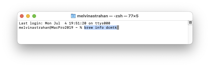
Be sure to make note of the Unix file path at which DCMTK was installed, it may differ slightly depending upon your version of Homebrew and MacOS. To determine where Homebrew installed the dcmtk package on your computer, in the Terminal application enter the command brew info dcmtk.
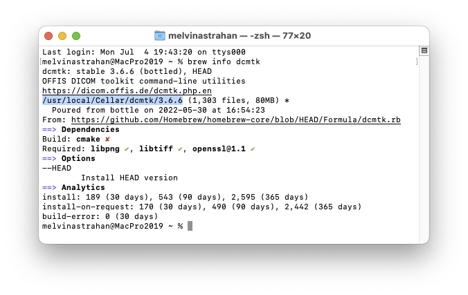
In my 2019 Intel Mac Pro, Homebrew installed the package at
/usr/local/Cellar/dcmtk/3.6.6
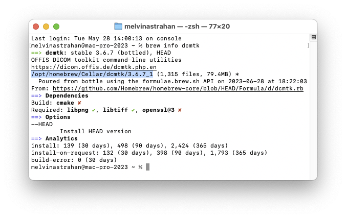
In my 2023 Apple Silicon Mac Pro M2-ultra, Homebrew installed the package at
/opt/homebrew/Cellar/dcmtk/3.6.7_1
Add
/bin to that path and enter the result in PS
Folders Preferences as:
For an Intel cpu Mac the file path is typically some variant of usr/local/....

For an Apple Silicon cpu Mac the file path is typically some variant of opt/homebrew/Cellar/....

Your installation may differ slightly from the above examples, e.g in 2024 you might install dcmtk version 3.6.8 instead of 3.6.7_1 that I installed in 2023.
If you have successfully installed DCMTK and PS can find it, the DCMTK indicator on the right of the MPR window toolbar will be green. If the indicator is red you will need to customize the file path to DCMTK in PS Folders Preferences. Click the indicator to take you to the folder preferences window.
With the DCMTK toolkit installed and located:
- Create a folder named DICOM (note: additional special folders named CT, MRI, DJPEG and DRLE are also allowed) somewhere other than in your patient folder's first hierarchical level and place within it your HFS AXIAL series of DICOM files (e.g. xxx.dcm). These .dcm files should use little endian DICOM Transfer Syntax UID (the default is tag 0002,0010 = 1.2.840.10008.1.2). Ideally, this folder should contain only the images that comprise a single imaging series. The MacOS Finder provides thumbnails of .dcm files which may help to quickly eliminate unnecessary files.
- Note: PS does NOT support pixel data that uses a compressed DICOM Transfer Syntax UID, but does provide a method to convert JPEG and RLE compressed pixel data to the expected default Transfer Syntax UID. If the pixel data in the DICOM files is JPEG compressed, launch PS and drag the DICOM folder onto the MPR window while holding down the option key. If the pixel data is RLE compressed, follow the same procedure except press the command key. PS will create a new folder in the same location as the original folder named DJPEG or DRLE that contains uncompressed versions of all the DICOM files that were found in the DICOM folder. This conversion is performed by the dcmdjpeg and dcmdrle functions that are part of the DCMTK toolkit.
- Launch PS and drag the DICOM folder (or intermediate DJPEG or DRLE folder if you created one to deal with compressed pixel data) onto the MPR window of PS6. PS6 will create a new folder (in the same location as the original folder) named DCMTK that contains .xml versions of all the DICOM files that were found in the DICOM (or DJPEG or DRLE) folder. This is done using the dcm2xml function that is part of the DCMTK toolkit.
- Drag the resulting DCMTK folder to the first hierarchical level your patient folder along with your other imaging files such as US1, US2, optomap, misc# and so on... If the DCMTK folder is available, there is no longer any need to manually create and export .jpg planar reconstructions such as Axial, Sagittal, Equator, t-Coronal and t-Meridan using OsiriX or Horus.
- You can either manually drag a DCMTK folder onto the MPR window to load its images, or if the DCMTK folder is located in the first hierarchical level of the patient folder along with the ophthalmology images you can simply drag the patient folder itself onto the Image window as usually done when intializing a new patient plan.
Alternatively, if you dont want to install DCMTK, you can create a folder named "RAW" into which 16-bit signed image data in .raw file format and a single DICOM meta-data file in .xml format have been exported from OsiriX. PS7 is expected to further streamline the import of most DICOM files but will still require installing the DCMTK toolkit.
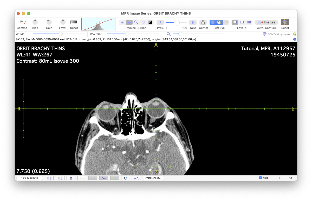
The Multi-Planar Reconstruction (MPR) window is used to manage the loading, display, and reconstructions derived from a 3D CT (or MRI) study series. The 3D study series is expected to consist of a head-first, supine (HFS) sequence of thin axial slices covering the orbits and including both eyes plus a few cm superior and inferior to the orbits. It is important that both eyes are included because ocular symmetry will be leveraged to help compensate for head rotations in the scanner. Slice spacing must be consistent and slice thickness as thin as possible (e.g. < 1mm). Image data must be 16-bit monochrome. Image dimensions should be 512x512 pixels.
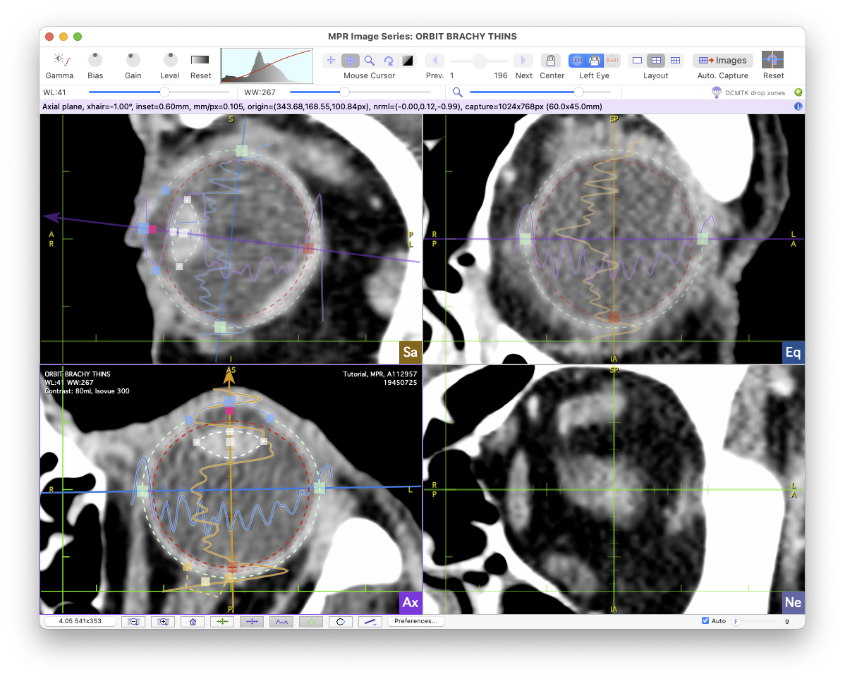
The status line just below the toolbar provides information about the currently selected layout pane.
In addition to the buttons in this window, other reconstruction parameters and access to DICOM meta-data are adjustable from the MPR menu which is added to the menu bar any time this window is frontmost.
The MPR window defaults to single pane layout mode. In this layout you can load a study series by dragging and dropping a folder of DICOM images that have been converted to .xml file format. The folder must be named DCMTK. In version 6.8.6 a study series may optionally be exported from OsiriX as raw pixel data but this is far more involved than using the DCMTK folder approach. Using OsiriX, export the study series to a folder named RAW which contains all of the pixel data data in .raw file format using OsiriX's Export->Raw... menu. In this RAW folder there must also be a single file containing representative DICOM metadata, exported from OsiriX's Meta-Data window in .xml file format (e.g. PatientName.xml).
Planar reconstructions are created by switching to 4 or 6 pane layout using the Layout control in the toolbar.
In 4 pane layout the planar reconstructions are:
- Upper left pane (Sa): Sagittal reconstruction.
- Lower left pane (Ax): Axial reconstruction.
- Upper right pane (Eq): Equator reconstruction.
- Lower right pane (Ne): Nerve-coronal reconstruction.
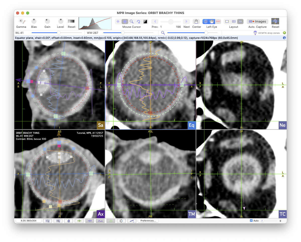
In six pane layout the planar reconstructions are:
- Upper left pane (Sa): Sagittal reconstruction.
- Lower left pane (Ax): Axial reconstruction.
- Upper middle pane (Eq): Equator reconstruction.
- Lower middle pane (TM): Tumor-meridian reconstruction.
- Upper right pane (Ne): Nerve-coronal reconstruction.
- Lower right pane (TC): Tumor-coronal reconstruction.
The meridian angle and coronal planar offsets from the equator automatically track those planes as they are defined and set in the
Planar Dosimetry window. The crosshair displayed in the axial, sagittal and equator is used to
find the geometric center (as defined by Plaque Simulator) of the eye. Fine tuning of the eye model will be accomplished by capturing these MPR window reconstructions (using the
Auto. Capture control) to Plaque Simulator's
Image window and proceeding as usual in that window.
The orthogonal MPR crosshairs includes 1 mm tick marks and an optional histogram of the gray levels of the pixels beneath the histogram axes. The outer sclera is designated by a dashed green oval. The surface for oblate-spheroid reconstructions (e.g. the inner surface of the sclera to map the tumor base) is designated by a dashed red oval. The basic dimensions of the eye and spherical reconstruction surface can be adjusted using the control handles found on the crosshair axes. In the example below you can see in the nerve-coronal reconstruction (upper-right pane) that the center of the optic nerve connects to the eye about 1 mm superior to the geometric axial bisecting plane.